Excel is powerful and does just about everything one could ask for in a spreadsheet. It’s not just for numbers. Plenty of people populate Excel’s seemingly infinite grids with data, using it as a flat-file database. It can make a relatively effective contact manager or full-blown customer relationship manager. Not to mention the almost infinite number of excellent-looking charts it can generate with the right (or even wrong!) data.

Paint Cells to a New Format

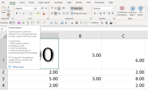
Let’s say you change not only the wrapping in a cell, but also the entire look—the font, the color, whatever. And you want to apply it to many, many other cells. The trick is the Format Painter tool, the one that is on the Home tab that looks like a paint brush.

Select the sell you like, click the icon, and then click on a different cell to paint in the format—they’ll match in looks, not in content. Want to apply it to multiple tabs? Double-click the paint brush icon, then click away on multiple cells.

Line Breaks and Wrapping Text

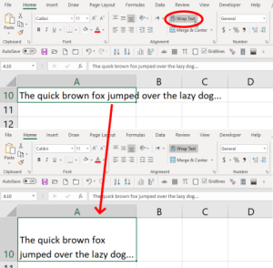
Typing into spreadsheet cells can be frustrating, as the default for text you type is to continue on forever, without wrapping back down to a new line. You can change that. Create a new line by typing Alt+Enter (hitting Enter alone takes you out of the cell). Or, click the Wrap Text option under the Home tab, which means all text wraps right at the edge of the cell you’re in. Resize the row/column and the text re-wraps to fit.

If you’ve got multiple cells that have text overruns, select them all before you click Wrap Text. Or, select all the cells before you even type in them and click Wrap Text. Then whatever you type will wrap in the future.

Autofit All the Columns/Rows Instantly

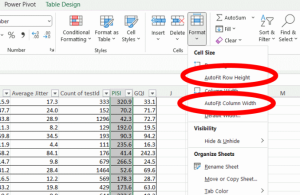
If you’ve got a sheet full of truncated cells (with no text wrap) that no one can read, manually clicking column and row headers one by one helps with readability, but could take a while. Instead, do a Ctrl+A to select all then tap Alt+HOI (hit the letters in that order). That will autofit all the columns. Then use Alt+HOA to autofit the rows. Every cell will be instantly readable, even if now you have to hit the scrollbar more to see everything on the sheet. You can also find those commands using Home > Format > Autofit Row Height or AutoFit Column Width.

AutoFill Your Cells

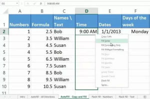
This is a no-brainer, but so easily overlooked. You start typing a series of repetitive things like dates (1/1/23, 1/2/23, 1/3/23, etc.) and you know you’re in for a long day. Instead, begin the series and move the cursor on the screen to the lower-right part of the last cell—the fill handle. When it turns into a plus sign (+), click and drag to select all the cells you need to fill. They’ll magically fill using the pattern you started. It can go up or down a column, or left or right on a row.

Even better—try Auto Fill without much of a pattern. Again, pick a cell or cells, move to the fill handle, right-click, and drag. You’ll get a menu of options. The more data you input at first, the better the Fill Series option will do creating your AutoFill options. Check out this Microsoft tutorial(Opens in a new window).

Flass Fill, Fastest Fill Alive

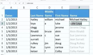
Flash Fill will smartly fill a column based on the pattern of data it sees in the first column (it helps if the top row is a unique header row). For example, if the first column is all phone numbers that are formatted like “21255554111” and you want them to all look like “(212)-555-4111,” start typing. By the second cell, Excel should recognize the pattern and display what it thinks you want. Just hit enter to use them.

This works with numbers, names, dates, etc. If the second cell doesn’t give you an accurate range, type some more—the pattern might be hard to recognize. Then go to the Data tab and click the Flash Fill button.

Ctrl+Shift to Select

There are much faster ways to select a dataset than using the mouse and dragging the cursor, especially in a spreadsheet that could contain hundreds of thousands of rows or columns. Click in the first cell you want to select and hold down Ctrl+Shift, then hit either the down arrow to get all the data in the column below, up arrow to get all the data above, or left or right arrow to get everything in the row (to the left or right, of course). Combine the directions, and you can get a whole column as well as everything in the rows on the left or right. It’ll only select cells with data (even invisible data).

If you use Ctrl+Shift+End, the cursor will jump to the lowest right-hand cell with data, selecting everything in between, even blank cells. So if the cursor is in the upper-left cell (A1), that’s everything.

Ctrl+Shift+* (the asterisk) might be faster, as it will select the whole contiguous data set of a worksheet, but it will stop at cells that are blank.

Text to Columns

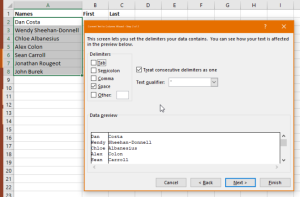
Say you’ve got a column full of names, first next to last, but you want two columns that break them out. Select the data, then on the Data tab (at the top) click Text to Columns. Choose to separate them by either delimiters (based on spaces or commas—great for CSV data values) or by a fixed width. Fixed width is utilized when all the data is crammed into the first column, but separated by a fixed number of spaces or period. The rest is like magic, with extra options for certain numbers.

We hope these tips have been helpful in your business.  Please let us know if you have any questions about your IT environment or how to secure it from outside cyber threats. Contact us at (732) 780-8615 or email at [email protected].

Eric Griffith, “32 Excel Tips for Becoming a spreadsheet Pro”, pcmag.com, Dec. 30, 2022